Early history of global atmospheric and climate modeling at NCAR
Enjoy this excerpt from Warren's autobiography, "Odyssey in Climate Modeling, Global Warming, and Advising Five Presidents"
(continued from page 1) weather predictability limits. The UCLA Medical School had an IBM 7090 computer and it was idle during the weekends. Yale Mintz had an arrangement with the Medical School staff that allowed his group to use the computer for numerical experiments with his UCLA model.
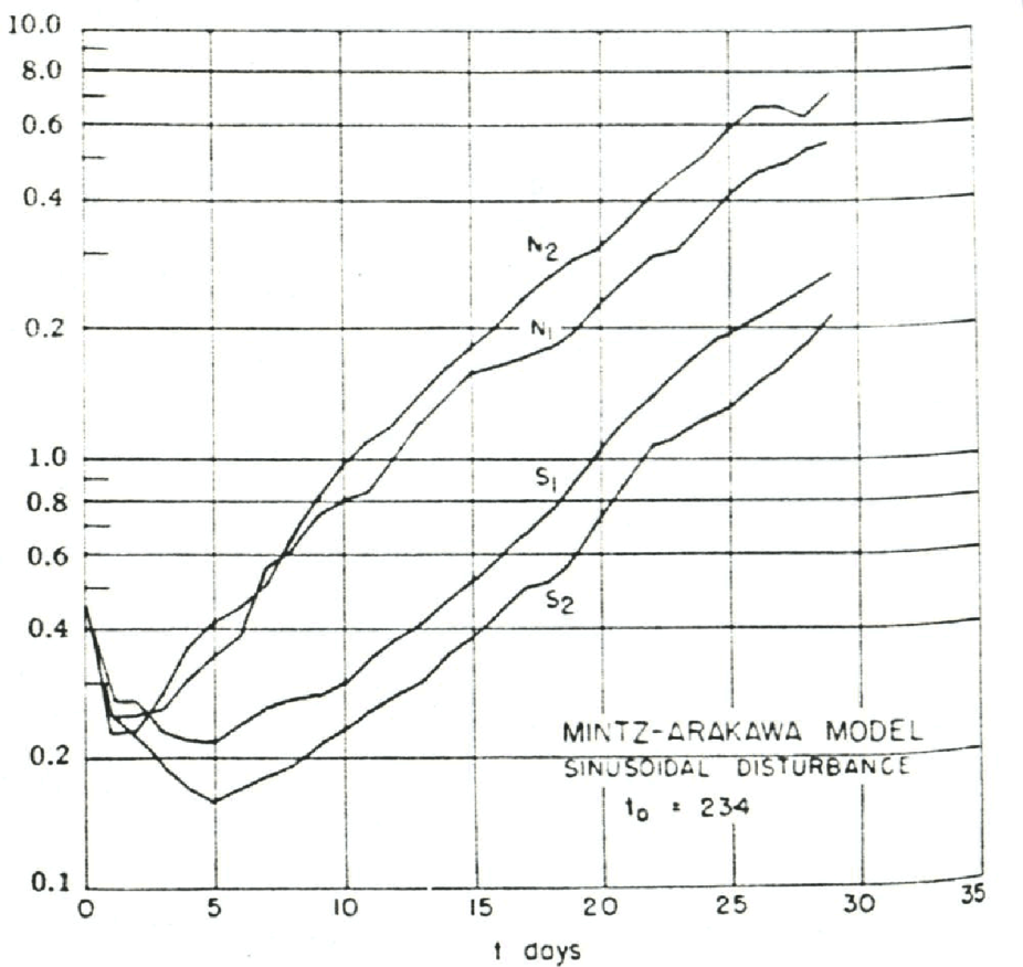
This figure shows the first error growth simulation with the Mintz-Arakawa atmospheric model. I plotted this graph on the day after I returned from helping run the model on the UCLA Medical School IBM 7090 computer. A small sinusoidal disturbance or perturbation, “the butterfly effect”, was added to the initial temperature data and the model was run and compared to another simulation without the perturbation. The root mean square error growth was plotted. The error grew rapidly and then started to level off near 30 days (not shown). At that time, the control and perturbation simulations looked entirely different. They had the same “climate” or time average properties but the detailed weather forecasts were entirely different. This provided the first estimate of how far into the future one could forecast the details of the weather.In order to start the experiments, we introduced a small perturbation into the model temperature data at a particular time of a previous long “control” experiment and we repeated the model experiment. This meant I had to stay up all Saturday night with the UCLA programmer. The small perturbation to the initial conditions began to grow as the calculation proceeded, as predicted by the “flap of butterfly wings” chaos theory that in our case was the small change in temperature. At the end of three or four weeks of simulation, the computer generated storm systems that formed in both hemispheres that were entirely different from those in the control experiment. I returned to Boulder late Sunday evening and the next day I plotted the root mean error data between the experiment with the small perturbation and the control experiment. I showed the plots to Charney and the others. It was clear that the growth of error seem to reach a maximum at about three weeks. Figure 6 shows that the error grew from a small value at day zero which grew out to 28 days and then started to level off.
With caution, we announced to our colleagues that we had found a theoretical limit to weather forecasts. Of course, over the years, many groups took part in this sort of exercise, but it is interesting to see that the fundamentals remained the same. It is probably impossible to make “detailed” forecasts of weather events past two or three weeks. Of course, it is now possible to perform useful ensemble forecasts for much longer periods…on the order of weeks to months in advance, and in some cases seasons ahead. However, these are more “statistical forecasts” instead of detailed deterministic forecasts of large-scale weather systems. In other words, the ensemble forecasts do not determine the paths of individual storms systems but an envelope for possible paths.
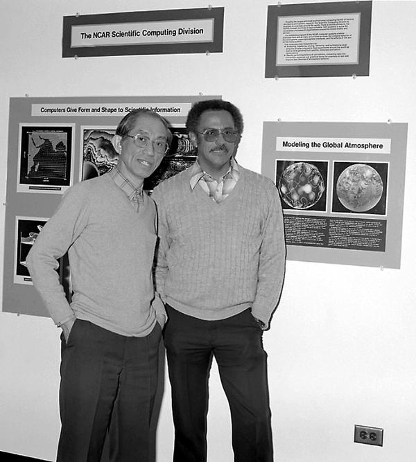
When Akira and I started to develop a General Circulation Model (GCM) in 1964, we decided to try a different approach. I will not go too deeply into the technical details3. We used height above the Earth’s surface as the coordinate in the vertical and latitude and longitude for the horizontal grid structure. The form of the equations followed closely those of the legendary Lewis Richardson (1922), who used a similar set of equations and solved the mathematics with a mechanical calculator. His attempt was pioneering, but not successful for several reasons, which are beyond the scope of this book. Richardson4 wrote a famous book, which outlined the fundamental methods of building weather and climate models5.
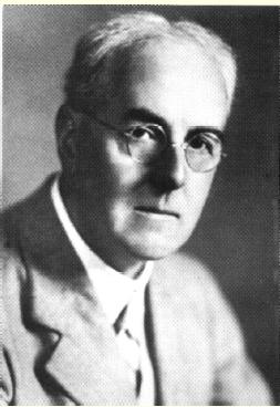
Lewis F. Richardson The NCAR model6 was constructed by a small team of scientists and computer programmers. The programmers included Bernie O’Lear, Gloria De Santo (who later married David Williamson), Joyce Takamine, and several others7. They did an excellent job of constructing the code and preparing the operational software to run on the early computers we had at that time. Typically, we would meet each weekday morning, look at the output from the experiment of the previous night or weekend, and then decide what needed fixing or changing. As time went on, the model became more stable and we were able to run longer simulations of the atmosphere. Even so, progress was slow, in part, because the computers were so slow. (continued, next page)
3 More detailed information on the development and use of NCAR’s GCMs can be found at http:/www.ucar.edu/archives/. The first paper was Kasahara and W. M. Washington, 1967: NCAR global general circulation model of the atmosphere, Monthly Weather Review, 95, 389-402.
4 In 1922, Lewis F. Richardson wrote an interesting and partly entertaining book on how he built an atmospheric model. He used a manual calculator for his pioneering attempt. Weather Prediction by Numerical Process. Cambridge University Press, xii+236 pp. It was reprinted by Dover Publications, New York, 1965, with a New Introduction by Sydney Chapman, xvi+236 pp. Also, a personal account of his life can be found in a book by Oliver Ashford: Prophet-or Professor?: The Life and Work of Lewis Fry Richardson, Adam Hilger Ltd, Bristol and Boston, 1985.
5 There are many books and scientific articles on climate models. The book written by the author and Claire Parkinson and NASA (An Introduction to Climate Modeling (2005, 2nd Edition), University Science Books) explains the basic history and fundamentals that are in climate models.
6 NCAR modeling history can be found in the NCAR Quarterly January 1963 and November 1971.
7 Larry Williams, Dave Robertson, Robert Wellck, Gerald Browning, Joseph Oliger, and Dave Kennison were some of early programmers who provided substantial support to the development of the models.