Early history of global atmospheric and climate modeling at NCAR
Enjoy this excerpt from Warren's autobiography, "Odyssey in Climate Modeling, Global Warming, and Advising Five Presidents"
(continued from page 2) In the mid-1960s, most of the emphasis was on simulating the hemispheric or global weather. The physical processes of radiation, clouds, precipitation, mountains, boundary fluxes between the atmosphere and the earth’s surface were extremely simple. There was strong support for building a general circulation model, but there was some advantage of not having too many “cooks in the kitchen.” We did not have the programming or computing capacity to try many different options.
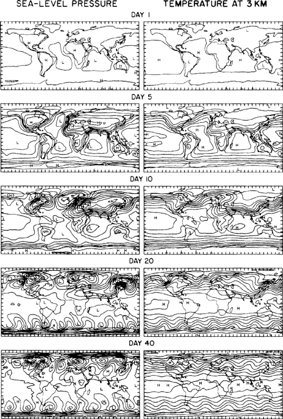
The time sequence of geographical distributions of sea level pressures and 3 km temperatures is shown from a perpetual January simulation of an early two-layer atmospheric GCM starting at rest with a 240 K isothermal atmosphere. The pressure contours are drawn at intervals of 4 mb and the temperature contours at intervals of five K. (From Washington 1968.). This was an exciting time for me. We were actually in the mid-1960s, starting to see the model generate more realistic storm systems and we were even able to display them on a cathode ray tube (CRT) device that was filmed by a camera. A time sequence of the state of the atmosphere is shown in Figure 68. At day 0, the model started with the atmosphere that had an artificial state of constant cold temperature over the entire globe and no motions. We specified the observed ocean temperatures and the placement of the major continents where the surface temperature was computed, based on a balance of surface radiation, latent heat (evaporation), and sensible heat fluxes between the atmosphere and the earth’s surface. The model allowed us to play “god”9 a bit in day 1 through 5. The atmosphere over the ocean strongly heats up, as shown on the right side of the figure and the continental areas cool. The associated sea-level pressure distribution at the earth’s surface is shown in the left panels. The model formed a monsoon pattern with sinking over the continents and rising motions over the oceans, where there is very strong heating. By day 10, the simple monsoon type systems started to break down and mid-latitude storm systems started to form. These storm systems are the typical low and high-pressure patterns that are seen on weather maps. Associated with each of the mid-latitude weather systems were cold fronts where cold and drier air is transported from the Polar Regions. In the opposite sense, the warm fronts brought warmer moist air from the subtropics to higher latitudes. By day 40, the atmospheric “climate” came into approximate equilibrium. The pattern of more varied weather systems in the northern hemisphere was caused by the continents, effecting the formation of areas of cool and warm temperatures depending on the season. The storm systems in the southern hemisphere were of similar strength because there were fewer large continents compared to the northern hemisphere, as is shown on the day 40 plots. Obviously, this very simple model from the mid-1960s has been greatly superseded by many generations of state-of-art climate models, with much increased resolution and more accurate and realistic treatments of physical processes such as clouds, convection, radiation, ocean, land-vegetation, and sea ice treatments.10
One of the purposes of NCAR was and still is to provide facilities such as computing and observing systems to the academic community that would be beyond the capabilities of a single university. In the same vein, the academic community needs to have tools such as a general circulation or climate models for its research. Although, there are presently successful models built at universities, they are not usually regarded as community tools and are not supported as such. It was then natural for NCAR, with its funding from the National Science Foundation and the Department of Energy, as well as its university collaborators, to build a family of climate models that could be used by a large community of scientists and computational experts. The science community needs to keep in mind that in order to remain at the state-of-art, there needs to be a scientific infrastructure at a place like NCAR to develop and improve tools like climate models. University scientists and graduate students are encouraged to explore novel and innovative solutions to many climate related problems with the models. I have always been an especially strong advocate for university and other scientists to be involved in the development and use of climate models.
Our group at NCAR was able to perform some of the first simulations of the Indian-Asia summer monsoon11, showing the general wind and precipitation patterns in that region, and to perform the first simulation of the last ice age12 atmospheric climate using some of the early models.
Kirk Bryan In the 1970s, there was new emphasis on climate modeling at NCAR. It was to extend the modeling to include ocean and sea ice. We hired a number of oceanographers including Albert (Bert) Semtner, who had earned a Ph.D from Princeton University, while working with Kirk Bryan (GFDL), the developer of the widely used ocean model at that time. Two other NCAR oceanographers, Bill Holland and Jim McWilliams, were also heavily engaged in ocean modeling; however, they concentrated primarily on the regional and smaller scales.
Our group interacted mostly with Semtner who had reprogrammed an earlier GFDL ocean model to make it easier to use. He also added several options that were not built into the original model. Over the years, Semtner has been a close collaborator with the group and a close friend. Semtner collaborated with Bob Chervin of NCAR to carry out the pioneering global ocean simulation. Their calculations included realistic coastlines and ocean bottom. The model had a resolution high enough to see eddy types of structures seen in the observed ocean.
Additionally, both Semtner and Chervin took advantage of the then state of art supercomputer to perform this feat. They were awarded the first annual Computerworld/Smithsonian Award for Breakthrough Computational Science in 1993. Earlier in 1988, they received the Cray13 Research Leadership Award for Breakthroughs in Science and the Gordon Bell Award for Parallelism. They later received the Cray Research Gigaflop Performance Award in 1989. I am proud to have collaborated with both of them on the building of early generation coupled climate models.”
...end of excerpt...
8 This figure was part of an article I wrote for SCIENCE JOURNAL, November 1968. P37-41. This journal is no longer publishing.
9 In the Bible there is reference in Genesis of God creating the heaven and earth in seven days.
10 There are many examples of more modern climate models that can be found in the Washington and Parkinson book, An Introduction to Three Dimensional Climate Modeling referred to earlier in a footnote. The second edition was published in 2005 by University Science Books.
11 Washington and Daggupaty, 1975, J. Appl.Meteor., 14,114-119.
12 Williams, Barry, and Washington, 1974, J. Appl. Meteor., 13, 305-317.
13 Over my career, I have interacted with Dave Blaskovich, who is excellent sales representative for supercomputers built by Cray and IBM. His wisdom and good sense have prevented disasters with unworkable supercomputer systems.